 Forecasting customer demand is an important and necessary part of the chain of calculations needed to optimize inventory stocking levels. There are a wide variety of techniques that can be used, making forecasting a confusing and sometimes difficult process. If your goal is to not only forecast demand but also stock inventory at optimal levels, then forecasting must be combined with inventory planning and replenishment optimization algorithms to reach the goals of higher service levels with less inventory.
This blog provides some basic information about viable inventory forecasting techniques. Forecasting is one of the key steps in inventory planning but not the only one. There are other key variables and processes that come into play in good supply chain replenishment planning including inventory rationalization and optimization.
Forecasting is an important part of inventory replenishment planning
 Modern inventory planning systems perform a statistical analysis of historical item usage patterns to predict future usage. Some also employ demand-sensing techniques using real-time data in addition to some historic demand. After calculating a new forecast, the systems determine optimal stocking levels. On a day-to-day basis, they compare actual inventory status with optimal stocking levels to decide what to order and when. Thus, forecasts are a fundamental piece of inventory planning. The more accurate and usable the forecasts, the better job the planning can do in making sure service levels are high enough with a minimum of inventory.
The starting point for forecasting is clean and reliable demand history data
Item demand history is usually taken from actual sales or item order or shipping data. However, some businesses are able to capture customer demand requests that may or may not be satisfied from stock.
For inventory planning, forecasting usually deals with a time series of monthly or weekly data. Many times there are high demand spikes that need to be reviewed. What caused the spikes? Some examples might be:
- A data entry error leading to an erroneous data point in the organization’s transaction system. This happens more frequently than one would imagine.
- A special promotion for the item leading to a heavy demand in the off-season month.
- A large new customer signed on and stocked its locations, an event likely to be repeated when other new customers sign on.
Abnormal history data like this can be identified by methods such as Statistical Process Control (Control Charts). Some systems automatically eliminate or dampen these “outliers” which is helpful but can also be problematic if the cause is not known by the planner. Others change their value to be in the expected range. A third approach is to identify the situation automatically and have a user/planner change the outlier history value to one that most reasonably acts as a guide for forecasting.
Forecasting techniques vary by type of demand
 The forecasting process must indicate what level of demand is expected, by month, and the demand variance (how much the demand might spike.) The expected demand indicates the inventory needed for the re-supply period. The variance leads to a calculation of the safety or buffer stock needed to cover demand surges.
Statistical analysis of historical demand generates forecasts with three components: level, trend, and seasonality.
Level
Some products are staples with a fairly steady demand month after month. A moving window average of the last x months of demand can give a good picture of the level of demand, which may have some gradual changes.
Trend Up or Down
Other products have a rising or falling “trend.” The moving window average tends to lag behind reality, so a regression analysis finding a best fit straight line through the data points can give a better forecast.
The straight line fit may be misleading, however, if the history values bounce around a lot. The regression fit will show a downward trend, but the history curve bounces so much you don’t know if this trend is real. In such a case, you need to be careful how quickly you reduce the inventory levels. A statistical calculation called the R2 test tells how much confidence we should have in the regression fit.
Seasonal Demand
 Many items have large demand at certain times of year and little or no demand at other times. For example, parts for lawn mower repairs have a large demand spring and early summer, and little demand over the winter. Air conditioners and parts will have a slightly later season. Trend analysis for these items will often show an upward or downward trend when the real underlying behavior is a change of season.
Seasonal demand is best modeled by observing the demand for each calendar month over several years of history. These monthly averages can be smoothed if seasonal changes are gradual. Some forecasters model the seasonal changes with a Fourier Series (general approach to model any periodic function), but this is usually overkill. Box-Jenkins analysis (also referred to as Autoregressive/Integrated/Moving Average, or ARIMA) is a powerful way to analyze periodic time series data. It is also overkill in general, as the period is almost always 12 months for inventory planning situations. In some applications other periods, such as end-of-quarter hockey sticks, may make the ARIMA approach more useful.
Combined Trend and Season Demand
An item may have both seasonal demand characteristics and an upward or downward trend. Thus, it can be useful to forecast with a combination of trend and season characteristics. A variety of approaches outside the scope of this paper can be used to do this. More history is required, at least three years to get an accurate representation and then using a multiplicative forecasting approach.
Low Volume Demand
Some situations, such as service parts usage, have a large number of items with very low demand rates. The inventory planning questions of interest for these are:
- Should I stock the item at all (carry on the Authorized Stocking List)?
- If so, should I stock 1 or 2 to make sure I meet needed service or fulfillment levels?
Figure 4 shows an example of an item with low usage. The item only had demand in 4 of the 12 months shown and a total demand of 5 units for the year. Forecasting an average demand of 5/12 per month can be confusing to end users. The more interesting way to look at the situation is to report the observed probability distribution, and then make a stocking decision based on the likelihood of having a demand for that item over the next period of time.
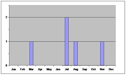
Figure 4. Low Volume Example
In the Figure 4 example, the historical usage suggests a demand probability distribution as follows:
- 8/12 = 2/3 probability of zero demand in a month
- 3/12 = ¼ probability of 1 demand in a month
- 1/12 probability of 2 demands in a month.
A low volume forecasting method employed in the past is Croston’s Method. It looks at the pattern of demand vs. non-demand months and how strong the demand was when it was non-zero. It then predicts that a similar pattern will repeat. This approach has been discredited for inventory planning, as it claims more definiteness for forecasted months than the situation warrants. For example, if the pattern suggests the next month should have zero demand, we might not stock the item in that month. But in reality, that month will have just as much chance of a demand as the following month that has a forecasted demand in the Croston’s model.
Next: Part Two covers forecast accuracy and forecasting problems. Learn more!
